How To Calculate Degeneracy Of Energy Levels

Energy level of a quantum system that corresponds to two or more different measurable states

In quantum mechanics, an free energy level is degenerate if it corresponds to two or more than different measurable states of a quantum organization. Conversely, two or more different states of a quantum mechanical system are said to be degenerate if they requite the same value of free energy upon measurement. The number of different states corresponding to a item energy level is known as the caste of degeneracy of the level. Information technology is represented mathematically by the Hamiltonian for the organisation having more one linearly contained eigenstate with the same energy eigenvalue.^[1] ^{: p. 48} When this is the instance, free energy lone is not enough to narrate what state the system is in, and other quantum numbers are needed to characterize the exact state when distinction is desired. In classical mechanics, this tin can be understood in terms of different possible trajectories corresponding to the same energy.

Degeneracy plays a central office in quantum statistical mechanics. For an $N$ -particle system in 3 dimensions, a single energy level may correspond to several different wave functions or energy states. These degenerate states at the same level all accept an equal probability of beingness filled. The number of such states gives the degeneracy of a particular free energy level.

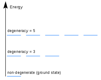
Degenerate states in a quantum system

Mathematics [edit]

The possible states of a quantum mechanical organization may be treated mathematically equally abstract vectors in a separable, circuitous Hilbert space, while the observables may be represented by linear Hermitian operators interim upon them. By selecting a suitable ground, the components of these vectors and the matrix elements of the operators in that basis may be determined. If $A$ is a $N \times Northward$ matrix, $X$ a non-zero vector, and $λ$ is a scalar, such that $AX=\lambda X$ , and so the scalar $λ$ is said to be an eigenvalue of $A$ and the vector $X$ is said to be the eigenvector respective to $λ$ . Together with the zero vector, the gear up of all eigenvectors corresponding to a given eigenvalue $λ$ grade a subspace of $C n$ , which is called the eigenspace of $λ$ . An eigenvalue $λ$ which corresponds to two or more different linearly independent eigenvectors is said to be degenerate, i.eastward., $AX_{1}=\lambda X_{one}$ and $AX_{2}=\lambda X_{2}$ , where $X_{1}$ and $X_{2}$ are linearly contained eigenvectors. The dimension of the eigenspace corresponding to that eigenvalue is known as its degree of degeneracy, which tin be finite or infinite. An eigenvalue is said to be not-degenerate if its eigenspace is one-dimensional.

The eigenvalues of the matrices representing physical observables in quantum mechanics give the measurable values of these observables while the eigenstates corresponding to these eigenvalues give the possible states in which the organisation may be found, upon measurement. The measurable values of the energy of a quantum arrangement are given by the eigenvalues of the Hamiltonian operator, while its eigenstates give the possible free energy states of the organisation. A value of free energy is said to be degenerate if there exist at to the lowest degree two linearly independent energy states associated with information technology. Moreover, whatsoever linear combination of 2 or more degenerate eigenstates is besides an eigenstate of the Hamiltonian operator corresponding to the aforementioned free energy eigenvalue. This clearly follows from the fact that the eigenspace of the energy value eigenvalue $λ$ is a subspace (being the kernel of the Hamiltonian minus $λ$ times the identity), hence is closed under linear combinations.

Proof of the to a higher place theorem.^[2] ^{: p. 52}

If ${\lid {H}}$ represents the Hamiltonian operator and $|\psi _{1}\rangle$ and $|\psi _{2}\rangle$ are two eigenstates corresponding to the aforementioned eigenvalue $East$ , and so

{\chapeau {H}}|\psi _{i}\rangle =Eastward|\psi _{1}\rangle

{\hat {H}}|\psi _{2}\rangle =Eastward|\psi _{two}\rangle

Let $|\psi \rangle =c_{1}|\psi _{1}\rangle +c_{two}|\psi _{2}\rangle$ , where $c_{1}$ and $c_{2}$ are complex(in general) constants, be whatever linear combination of $|\psi _{1}\rangle$ and $|\psi _{2}\rangle$ . Then,

{\begin{aligned}{\lid {H}}|\psi \rangle &={\chapeau {H}}(c_{1}|\psi _{1}\rangle +c_{two}|\psi _{2}\rangle )\\&=c_{ane}{\lid {H}}|\psi _{i}\rangle +c_{ii}{\hat {H}}|\psi _{2}\rangle \\&=East(c_{one}|\psi _{one}\rangle +c_{2}|\psi _{2}\rangle )\\&=E|\psi \rangle \end{aligned}}

which shows that $|\psi \rangle$ is an eigenstate of ${\hat {H}}$ with the same eigenvalue $E$ .

Result of degeneracy on the measurement of free energy [edit]

In the absenteeism of degeneracy, if a measured value of energy of a quantum organisation is adamant, the corresponding land of the organization is assumed to be known, since simply 1 eigenstate corresponds to each free energy eigenvalue. Even so, if the Hamiltonian ${\hat {H}}$ has a degenerate eigenvalue $E_{north}$ of degree g_n, the eigenstates associated with information technology form a vector subspace of dimension yard_north. In such a case, several concluding states can be mayhap associated with the same effect $E_{n}$ , all of which are linear combinations of the g_n orthonormal eigenvectors $|E_{north,i}\rangle$ .

In this case, the probability that the energy value measured for a system in the land $|\psi \rangle$ will yield the value $E_{n}$ is given by the sum of the probabilities of finding the system in each of the states in this basis, i.e.

P(E_{north})=\sum _{i=one}^{g_{due north}}|\langle E_{n,i}|\psi \rangle |^{2}

Degeneracy in unlike dimensions [edit]

This department intends to illustrate the existence of degenerate energy levels in quantum systems studied in different dimensions. The report of one and two-dimensional systems aids the conceptual understanding of more complex systems.

Degeneracy in one dimension [edit]

In several cases, analytic results can be obtained more easily in the study of one-dimensional systems. For a breakthrough particle with a wave role $|\psi \rangle$ moving in a 1-dimensional potential $Five(x)$ , the time-contained Schrödinger equation can be written as

-{\frac {\hbar ^{2}}{2m}}{\frac {d^{2}\psi }{dx^{2}}}+Five\psi =E\psi

Since this is an ordinary differential equation, at that place are ii independent eigenfunctions for a given energy $E$ at most, so that the degree of degeneracy never exceeds two. It can exist proven that in i dimension, there are no degenerate bound states for normalizable wave functions. A sufficient condition on a piecewise continuous potential $V$ and the energy $Eastward$ is the being of ii existent numbers $Thousand,x_{0}$ with $M\neq 0$ such that $\forall x>x_{0}$ we have $Five(x)-E\geq M^{2}$ .^[3] In particular, $V$ is bounded below in this criterion.

Proof of the to a higher place theorem.

Considering a 1-dimensional breakthrough arrangement in a potential

5(10)

with degenerate states

|\psi _{1}\rangle

and

|\psi _{2}\rangle

corresponding to the same free energy eigenvalue

E

, writing the time-independent Schrödinger equation for the system:

-{\frac {\hbar ^{2}}{2m}}{\frac {d^{ii}\psi _{1}}{dx^{2}}}+V\psi _{1}=E\psi _{1}

-{\frac {\hbar ^{ii}}{2m}}{\frac {d^{ii}\psi _{ii}}{dx^{2}}}+V\psi _{two}=E\psi _{2}

Multiplying the first equation by $\psi _{2}$ and the 2nd by $\psi _{one}$ and subtracting one from the other, we get:

\psi _{one}{\frac {d^{two}}{dx^{2}}}\psi _{2}-\psi _{ii}{\frac {d^{2}}{dx^{2}}}\psi _{1}=0

Integrating both sides

\psi _{i}{\frac {d\psi _{2}}{dx}}-\psi _{two}{\frac {d\psi _{ane}}{dx}}={\mbox{constant}}

In example of well-defined and normalizable moving ridge functions, the higher up abiding vanishes, provided both the wave functions vanish at at to the lowest degree one point, and we detect: $\psi _{1}(x)=c\psi _{2}(10)$ where $c$ is, in general, a complex constant. For bound state eigenfunctions (which tend to nix equally $x\rightarrow \infty$ ), and assuming $V$ and $E$ satisfy the condition given above, it tin can be shown^[iii] that also the first derivative of the wave function approaches cipher in the limit $ten\to \infty$ , so that the above abiding is zero and we have no degeneracy.

Degeneracy in two-dimensional quantum systems [edit]

Ii-dimensional quantum systems exist in all 3 states of matter and much of the variety seen in three dimensional thing can be created in two dimensions. Existent two-dimensional materials are made of monoatomic layers on the surface of solids. Some examples of two-dimensional electron systems accomplished experimentally include MOSFET, two-dimensional superlattices of Helium, Neon, Argon, Xenon etc. and surface of liquid Helium. The presence of degenerate free energy levels is studied in the cases of particle in a box and two-dimensional harmonic oscillator, which act as useful mathematical models for several real world systems.

Particle in a rectangular plane [edit]

Consider a free particle in a plane of dimensions $L_{x}$ and $L_{y}$ in a airplane of impenetrable walls. The time-independent Schrödinger equation for this system with wave function $|\psi \rangle$ can be written as

-{\frac {\hbar ^{2}}{2m}}\left({\frac {\fractional ^{2}\psi }{{\fractional x}^{ii}}}+{\frac {\partial ^{2}\psi }{{\partial y}^{2}}}\right)=Eastward\psi

The permitted energy values are

E_{n_{x},n_{y}}={\frac {\pi ^{2}\hbar ^{ii}}{2m}}\left({\frac {n_{ten}^{2}}{L_{x}^{2}}}+{\frac {n_{y}^{two}}{L_{y}^{two}}}\correct)

The normalized moving ridge function is

\psi _{n_{10},n_{y}}(x,y)={\frac {ii}{\sqrt {L_{x}L_{y}}}}\sin \left({\frac {n_{10}\pi x}{L_{ten}}}\right)\sin \left({\frac {n_{y}\pi y}{L_{y}}}\correct)

where $n_{x},n_{y}=1,2,3...$

So, quantum numbers $n_{ten}$ and $n_{y}$ are required to describe the energy eigenvalues and the lowest energy of the organisation is given past

E_{1,ane}=\pi ^{ii}{\frac {\hbar ^{two}}{2m}}\left({\frac {1}{L_{x}^{2}}}+{\frac {1}{L_{y}^{2}}}\correct)

For some commensurate ratios of the 2 lengths $L_{ten}$ and $L_{y}$ , certain pairs of states are degenerate. If $L_{x}/L_{y}=p/q$ , where p and q are integers, the states $(n_{x},n_{y})$ and $(pn_{y}/q,qn_{x}/p)$ accept the same energy and then are degenerate to each other.

Particle in a square box [edit]

In this example, the dimensions of the box $L_{x}=L_{y}=L$ and the energy eigenvalues are given past

E_{n_{x},n_{y}}={\frac {\pi ^{ii}\hbar ^{two}}{2mL^{2}}}(n_{x}^{2}+n_{y}^{2})

Since $n_{ten}$ and $n_{y}$ can be interchanged without changing the energy, each energy level has a degeneracy of at least 2 when $n_{ten}$ and $n_{y}$ are different. Degenerate states are also obtained when the sum of squares of breakthrough numbers corresponding to unlike free energy levels are the same. For example, the three states (northward_x = vii, northward_y = 1), (due north_x = 1, north_y = vii) and (n_x = n_y = 5) all take $East=50{\frac {\pi ^{2}\hbar ^{two}}{2mL^{ii}}}$ and constitute a degenerate set.

Degrees of degeneracy of different energy levels for a particle in a square box:

$n_{x}$	$n_{y}$	$E\left({\frac {\hbar ^{two}\pi ^{2}}{2mL^{ii}}}\correct)$	Degeneracy
i	1	2	1
2 ane	1 2	5 5	two
2	ii	viii	1
3 1	one iii	10 x	2
3 2	ii 3	thirteen 13	2
iv i	ane 4	17 17	2
iii	3	18	1
...	...	...	...
7 5 one	i five 7	l 50 50	3
...	...	...	...
8 7 4 1	1 iv seven viii	65 65 65 65	four
...	...	...	...
9 7 6 two	ii 6 seven nine	85 85 85 85	four
...	...	...	...
xi 10 five two	2 5 10 11	125 125 125 125	iv
...	...	...	...
14 x 2	2 x fourteen	200 200 200	3
...	...	...	...
17 13 vii	vii xiii 17	338 338 338	3

Particle in a cubic box [edit]

In this instance, the dimensions of the box $L_{x}=L_{y}=L_{z}=L$ and the energy eigenvalues depend on three quantum numbers.

E_{n_{x},n_{y},n_{z}}={\frac {\pi ^{2}\hbar ^{2}}{2mL^{2}}}(n_{x}^{2}+n_{y}^{2}+n_{z}^{2})

Since $n_{x}$ , $n_{y}$ and $n_{z}$ can exist interchanged without changing the energy, each energy level has a degeneracy of at least iii when the three quantum numbers are not all equal.

Finding a unique eigenbasis in case of degeneracy [edit]

If two operators ${\lid {A}}$ and ${\hat {B}}$ commute, i.e. $[{\hat {A}},{\hat {B}}]=0$ , then for every eigenvector $|\psi \rangle$ of ${\hat {A}}$ , ${\hat {B}}|\psi \rangle$ is also an eigenvector of ${\hat {A}}$ with the same eigenvalue. Even so, if this eigenvalue, say $\lambda$ , is degenerate, information technology tin be said that ${\lid {B}}|\psi \rangle$ belongs to the eigenspace $E_{\lambda }$ of ${\hat {A}}$ , which is said to exist globally invariant under the action of ${\chapeau {B}}$ .

For two commuting observables A and B, one can construct an orthonormal footing of the state space with eigenvectors common to the ii operators. Nevertheless, $\lambda$ is a degenerate eigenvalue of ${\hat {A}}$ , then it is an eigensubspace of ${\lid {A}}$ that is invariant under the action of ${\chapeau {B}}$ , so the representation of ${\hat {B}}$ in the eigenbasis of ${\lid {A}}$ is not a diagonal but a block diagonal matrix, i.due east. the degenerate eigenvectors of ${\hat {A}}$ are not, in general, eigenvectors of ${\hat {B}}$ . Withal, it is always possible to choose, in every degenerate eigensubspace of ${\lid {A}}$ , a footing of eigenvectors common to ${\lid {A}}$ and ${\hat {B}}$ .

Choosing a complete set of commuting observables [edit]

If a given observable A is non-degenerate, there exists a unique footing formed past its eigenvectors. On the other manus, if one or several eigenvalues of ${\chapeau {A}}$ are degenerate, specifying an eigenvalue is non sufficient to characterize a basis vector. If, by choosing an observable ${\hat {B}}$ , which commutes with ${\hat {A}}$ , information technology is possible to construct an orthonormal ground of eigenvectors common to ${\chapeau {A}}$ and ${\hat {B}}$ , which is unique, for each of the possible pairs of eigenvalues {a,b}, then ${\chapeau {A}}$ and ${\hat {B}}$ are said to form a consummate ready of commuting observables. However, if a unique fix of eigenvectors can even so not be specified, for at least one of the pairs of eigenvalues, a third observable ${\hat {C}}$ , which commutes with both ${\lid {A}}$ and ${\hat {B}}$ can be found such that the three class a complete set of commuting observables.

It follows that the eigenfunctions of the Hamiltonian of a quantum system with a mutual free energy value must be labelled by giving some additional information, which can be done by choosing an operator that commutes with the Hamiltonian. These additional labels required naming of a unique energy eigenfunction and are usually related to the constants of movement of the arrangement.

Degenerate energy eigenstates and the parity operator [edit]

The parity operator is defined by its action in the $|r\rangle$ representation of changing r to −r, i.e.

\langle r|P|\psi \rangle =\psi (-r)

The eigenvalues of P tin exist shown to exist limited to $\pm ane$ , which are both degenerate eigenvalues in an infinite-dimensional land infinite. An eigenvector of P with eigenvalue +ane is said to be even, while that with eigenvalue −1 is said to be odd.

Now, an fifty-fifty operator ${\hat {A}}$ is 1 that satisfies,

{\tilde {A}}=P{\hat {A}}P

[P,{\lid {A}}]=0

while an odd operator ${\hat {B}}$ is ane that satisfies

P{\lid {B}}+{\lid {B}}P=0

Since the square of the momentum operator ${\hat {p}}^{2}$ is fifty-fifty, if the potential V(r) is fifty-fifty, the Hamiltonian ${\hat {H}}$ is said to exist an even operator. In that case, if each of its eigenvalues are non-degenerate, each eigenvector is necessarily an eigenstate of P, and therefore it is possible to wait for the eigenstates of ${\hat {H}}$ among fifty-fifty and odd states. All the same, if i of the energy eigenstates has no definite parity, it can be asserted that the corresponding eigenvalue is degenerate, and $P|\psi \rangle$ is an eigenvector of ${\hat {H}}$ with the same eigenvalue as $|\psi \rangle$ .

Degeneracy and symmetry [edit]

The concrete origin of degeneracy in a quantum-mechanical system is ofttimes the presence of some symmetry in the system. Studying the symmetry of a quantum system can, in some cases, enable us to find the free energy levels and degeneracies without solving the Schrödinger equation, hence reducing attempt.

Mathematically, the relation of degeneracy with symmetry can be antiseptic every bit follows. Consider a symmetry performance associated with a unitary operator $S$ . Under such an operation, the new Hamiltonian is related to the original Hamiltonian by a similarity transformation generated past the operator $S$ , such that $H'=SHS^{-1}=SHS^{\dagger }$ , since $S$ is unitary. If the Hamiltonian remains unchanged nether the transformation operation $S$ , we take

SHS^{\dagger }=H

SHS^{-one}=H

HS=SH

[S,H]=0

Now, if $|\alpha \rangle$ is an free energy eigenstate,

H|\alpha \rangle =E|\alpha \rangle

where Due east is the corresponding energy eigenvalue.

HS|\alpha \rangle =SH|\alpha \rangle =SE|\blastoff \rangle =ES|\alpha \rangle

which means that $S|\blastoff \rangle$ is also an energy eigenstate with the aforementioned eigenvalue $Due east$ . If the two states $|\alpha \rangle$ and $S|\alpha \rangle$ are linearly independent (i.due east. physically distinct), they are therefore degenerate.

In cases where $S$ is characterized by a continuous parameter $\epsilon$ , all states of the course $S(\epsilon )|\blastoff \rangle$ accept the same energy eigenvalue.

Symmetry group of the Hamiltonian [edit]

The set of all operators which commute with the Hamiltonian of a breakthrough system are said to form the symmetry group of the Hamiltonian. The commutators of the generators of this group make up one's mind the algebra of the group. An n-dimensional representation of the Symmetry group preserves the multiplication table of the symmetry operators. The possible degeneracies of the Hamiltonian with a particular symmetry grouping are given by the dimensionalities of the irreducible representations of the grouping. The eigenfunctions respective to a due north-fold degenerate eigenvalue form a basis for a n-dimensional irreducible representation of the Symmetry grouping of the Hamiltonian.

Types of degeneracy [edit]

Degeneracies in a quantum organization can be systematic or accidental in nature.

Systematic or essential degeneracy [edit]

This is also called a geometrical or normal degeneracy and arises due to the presence of some kind of symmetry in the system under consideration, i.e. the invariance of the Hamiltonian under a certain performance, every bit described above. The representation obtained from a normal degeneracy is irreducible and the corresponding eigenfunctions form a basis for this representation.

Adventitious degeneracy [edit]

Information technology is a type of degeneracy resulting from some special features of the system or the functional grade of the potential under consideration, and is related perchance to a hidden dynamical symmetry in the system.^[4] It as well results in conserved quantities, which are ofttimes non easy to identify. Adventitious symmetries lead to these additional degeneracies in the discrete energy spectrum. An accidental degeneracy can be due to the fact that the group of the Hamiltonian is not consummate. These degeneracies are connected to the beingness of bound orbits in classical Physics.

Examples: Coulomb and Harmonic Oscillator potentials [edit]

For a particle in a central $1/ r$ potential, the Laplace–Runge–Lenz vector is a conserved quantity resulting from an adventitious degeneracy, in addition to the conservation of angular momentum due to rotational invariance.

For a particle moving on a cone under the influence of $i/ r$ and $r 2$ potentials, centred at the tip of the cone, the conserved quantities corresponding to accidental symmetry volition be 2 components of an equivalent of the Runge-Lenz vector, in add-on to one component of the angular momentum vector. These quantities generate SU(two) symmetry for both potentials.

Case: Particle in a abiding magnetic field [edit]

A particle moving under the influence of a constant magnetic field, undergoing cyclotron motion on a circular orbit is another important example of an accidental symmetry. The symmetry multiplets in this example are the Landau levels which are infinitely degenerate.

Examples [edit]

The hydrogen atom [edit]

In atomic physics, the jump states of an electron in a hydrogen atom show the states useful examples of degeneracy. In this example, the Hamiltonian commutes with the full orbital angular momentum ${\chapeau {Fifty^{2}}}$ , its component forth the z-direction, ${\hat {L_{z}}}$ , total spin angular momentum ${\chapeau {S^{ii}}}$ and its z-component ${\hat {S_{z}}}$ . The quantum numbers respective to these operators are $50$ , $m_{l}$ , $s$ (always i/ii for an electron) and $m_{s}$ respectively.

The energy levels in the hydrogen atom depend only on the principal quantum number $north$ . For a given $northward$ , all the states respective to $l=0,\ldots ,due north-i$ accept the same free energy and are degenerate. Similarly for given values of $north$ and $l$ , the $(2l+ane)$ , states with $m_{50}=-l,\ldots ,fifty$ are degenerate. The degree of degeneracy of the free energy level E_n is therefore : $\sum _{fifty\mathop {=} 0}^{northward-1}(2l+one)=northward^{two}$ , which is doubled if the spin degeneracy is included.^[i] ^{: p. 267f}

The degeneracy with respect to $m_{l}$ is an essential degeneracy which is present for whatsoever central potential, and arises from the absence of a preferred spatial direction. The degeneracy with respect to $l$ is often described as an adventitious degeneracy, but information technology can be explained in terms of special symmetries of the Schrödinger equation which are simply valid for the hydrogen atom in which the potential energy is given by Coulomb's police.^[one] ^{: p. 267f}

Isotropic three-dimensional harmonic oscillator [edit]

It is a spinless particle of mass thou moving in three-dimensional space, subject to a central forcefulness whose absolute value is proportional to the distance of the particle from the centre of force.

F=-kr

It is said to be isotropic since the potential $Five(r)$ interim on it is rotationally invariant, i.due east. : $5(r)=i/2\left(m\omega ^{two}r^{two}\correct)$

where $\omega$ is the angular frequency given past ${\textstyle {\sqrt {k/g}}}$ .

Since the state space of such a particle is the tensor product of the state spaces associated with the private one-dimensional moving ridge functions, the time-independent Schrödinger equation for such a system is given by-

-{\frac {\hbar ^{2}}{2m}}\left({\frac {\fractional ^{2}\psi }{\partial x^{2}}}+{\frac {\fractional ^{2}\psi }{\fractional y^{2}}}+{\frac {\partial ^{2}\psi }{\partial z^{ii}}}\right)+{\frac {1}{two}}{m\omega ^{2}(x^{2}+y^{2}+z^{2})\psi }=Eastward\psi

And so, the energy eigenvalues are $E_{n_{10},n_{y},n_{z}}=(n_{x}+n_{y}+n_{z}+iii/2)\hbar \omega$

or, $E_{n}=(n+3/2)\hbar \omega$

where n is a non-negative integer. And then, the energy levels are degenerate and the degree of degeneracy is equal to the number of dissimilar sets $\{n_{ten},n_{y},n_{z}\}$ satisfying

n_{x}+n_{y}+n_{z}=n

The degeneracy of the $n$ -thursday state can exist found by because the distribution of $north$ quanta beyond $n_{x}$ , $n_{y}$ and $n_{z}$ . Having 0 in $n_{ten}$ gives $due north+one$ possibilities for distribution across $n_{y}$ and $n_{z}$ . Having 1 quanta in $n_{ten}$ gives $n$ possibilities across $n_{y}$ and $n_{z}$ and and then on. This leads to the full general issue of $n-n_{x}+1$ and summing over all $n$ leads to the degeneracy of the $n$ -th country,

\sum _{n_{10}=0}^{north}(due north-n_{ten}+1)={\frac {(n+ane)(northward+two)}{2}}

As shown, just the footing state where $northward=0$ is not-degenerate (ie, has a degeneracy of $one$ ).

Removing degeneracy [edit]

The degeneracy in a quantum mechanical organization may exist removed if the underlying symmetry is broken by an external perturbation. This causes splitting in the degenerate energy levels. This is essentially a splitting of the original irreducible representations into lower-dimensional such representations of the perturbed organisation.

Mathematically, the splitting due to the application of a small-scale perturbation potential can be calculated using time-independent degenerate perturbation theory. This is an approximation scheme that can exist applied to find the solution to the eigenvalue equation for the Hamiltonian H of a quantum organization with an applied perturbation, given the solution for the Hamiltonian H₀ for the unperturbed organisation. It involves expanding the eigenvalues and eigenkets of the Hamiltonian H in a perturbation series. The degenerate eigenstates with a given free energy eigenvalue form a vector subspace, but not every basis of eigenstates of this space is a good starting indicate for perturbation theory, because typically there would not be any eigenstates of the perturbed arrangement near them. The correct ground to cull is one that diagonalizes the perturbation Hamiltonian within the degenerate subspace.

Lifting of degeneracy past starting time-order degenerate perturbation theory.

Consider an unperturbed Hamiltonian

{\lid {H_{0}}}

and perturbation

{\lid {V}}

, so that the perturbed Hamiltonian

{\chapeau {H}}={\lid {H_{0}}}+{\hat {5}}

The perturbed eigenstate, for no degeneracy, is given by-

|\psi _{0}\rangle =|n_{0}\rangle +\sum _{k\neq 0}V_{k0}/(E_{0}-E_{chiliad})|n_{grand}\rangle

The perturbed energy eigenket as well equally higher order energy shifts diverge when $E_{0}=E_{k}$ , i.eastward., in the presence of degeneracy in energy levels. Assuming ${\hat {H_{0}}}$ possesses Northward degenerate eigenstates $|m\rangle$ with the same free energy eigenvalue E, and besides in full general some non-degenerate eigenstates. A perturbed eigenstate $|\psi _{j}\rangle$ tin can be written as a linear expansion in the unperturbed degenerate eigenstates equally-

|\psi _{j}\rangle =\sum _{i}|m_{i}\rangle \langle m_{i}|\psi _{j}\rangle =\sum _{i}c_{ji}|m_{i}\rangle

[{\hat {H_{0}}}+{\hat {V}}]\psi _{j}\rangle =[{\hat {H_{0}}}+{\hat {V}}]\sum _{i}c_{ji}|m_{i}\rangle =E_{j}\sum _{i}c_{ji}|m_{i}\rangle

where $E_{j}$ refer to the perturbed energy eigenvalues. Since $E$ is a degenerate eigenvalue of ${\hat {H_{0}}}$ ,

\sum _{i}c_{ji}{\chapeau {V}}|m_{i}\rangle =(E_{j}-E)\sum _{i}c_{ji}|m_{i}\rangle =\Delta E_{j}\sum _{i}c_{ji}|m_{i}\rangle

Premultiplying past another unperturbed degenerate eigenket $\langle m_{k}|$ gives-

\sum _{i}c_{ji}[\langle m_{1000}|{\chapeau {V}}|m_{i}\rangle -\delta _{ik}(E_{j}-E)]=0

This is an eigenvalue problem, and writing $V_{ik}=\langle m_{i}|{\hat {V}}|m_{m}\rangle$ , we have-

{\begin{vmatrix}V_{11}-\Delta E_{j}&V_{12}&\dots &V_{1N}\\V_{21}&V_{22}-\Delta E_{j}&\dots &V_{2N}\\\vdots &\vdots &\ddots &\vdots \\V_{N1}&V_{N2}&\dots &V_{NN}-\Delta E_{j}\end{vmatrix}}.\,

The N eigenvalues obtained past solving this equation give the shifts in the degenerate energy level due to the applied perturbation, while the eigenvectors give the perturbed states in the unperturbed degenerate basis $|m\rangle$ . To choose the good eigenstates from the outset, it is useful to notice an operator ${\lid {Five}}$ which commutes with the original Hamiltonian ${\lid {H_{0}}}$ and has simultaneous eigenstates with information technology.

Physical examples of removal of degeneracy by a perturbation [edit]

Some of import examples of physical situations where degenerate free energy levels of a quantum system are split up by the application of an external perturbation are given below.

Symmetry breaking in ii-level systems [edit]

A two-level system substantially refers to a physical organization having two states whose energies are close together and very different from those of the other states of the system. All calculations for such a system are performed on a two-dimensional subspace of the state space.

If the basis country of a physical organization is two-fold degenerate, any coupling between the two corresponding states lowers the energy of the ground state of the system, and makes information technology more stable.

If $E_{i}$ and $E_{2}$ are the energy levels of the system, such that $E_{1}=E_{two}=Eastward$ , and the perturbation $Westward$ is represented in the two-dimensional subspace as the following ii×2 matrix

\mathbf {Westward} ={\begin{bmatrix}0&W_{12}\\W_{12}^{*}&0\end{bmatrix}}.

and then the perturbed energies are

E_{+}=E+|W_{12}|

E_{-}=E-|W_{12}|

Examples of two-state systems in which the degeneracy in energy states is cleaved past the presence of off-diagonal terms in the Hamiltonian resulting from an internal interaction due to an inherent holding of the organization include:

Benzene, with two possible dispositions of the three double bonds between neighbouring Carbon atoms.
Ammonia molecule, where the Nitrogen atom can exist either above or below the plane defined by the three Hydrogen atoms.
H ⁺
₂ molecule, in which the electron may be localized around either of the two nuclei.

Fine-structure splitting [edit]

The corrections to the Coulomb interaction between the electron and the proton in a Hydrogen cantlet due to relativistic motion and spin–orbit coupling outcome in breaking the degeneracy in free energy levels for different values of l corresponding to a single main quantum number northward.

The perturbation Hamiltonian due to relativistic correction is given by

H_{r}=-p^{4}/8m^{3}c^{2}

where $p$ is the momentum operator and $m$ is the mass of the electron. The first-order relativistic energy correction in the $|nlm\rangle$ basis is given past

E_{r}=(-1/8m^{3}c^{2})\langle nlm|p^{4}|nlm\rangle

Now $p^{iv}=4m^{2}(H^{0}+eastward^{2}/r)^{ii}$

{\begin{aligned}E_{r}&=(-1/2mc^{two})[E_{n}^{2}+2E_{due north}e^{2}\langle 1/r\rangle +e^{4}\langle 1/r^{2}\rangle ]\\&=(-1/2)mc^{2}\alpha ^{four}[-3/(4n^{iv})+1/{n^{3}(l+1/two)}]\finish{aligned}}

where $\alpha$ is the fine construction abiding.

The spin–orbit interaction refers to the interaction betwixt the intrinsic magnetic moment of the electron with the magnetic field experienced by it due to the relative motion with the proton. The interaction Hamiltonian is

H_{then}=-(e/mc){{\vec {k}}\cdot {\vec {50}}/r^{three}}=[(east^{2}/(m^{two}c^{ii}r^{3})){\vec {S}}\cdot {\vec {L}}]

which may be written as

H_{so}=(east^{ii}/(4m^{2}c^{2}r^{3}))[{\vec {J}}^{ii}-{\vec {L}}^{2}-{\vec {S}}^{two}]

The start order free energy correction in the $|j,chiliad,fifty,1/2\rangle$ footing where the perturbation Hamiltonian is diagonal, is given by

E_{so}=(\hbar ^{2}due east^{2})/(4m^{two}c^{2})[j(j+1)-l(fifty+1)-three/iv]/((a_{0})^{3}n^{iii}(l(50+1/2)(fifty+1))]

where $a_{0}$ is the Bohr radius. The total fine-structure free energy shift is given by

E_{fs}=-(mc^{2}\alpha ^{4}/(2n^{3}))[ane/(j+1/2)-3/4n]

for $j=l\pm 1/2$ .

Zeeman effect [edit]

The splitting of the energy levels of an atom when placed in an external magnetic field because of the interaction of the magnetic moment ${\vec {thousand}}$ of the atom with the applied field is known as the Zeeman outcome.

Taking into consideration the orbital and spin angular momenta, ${\vec {Fifty}}$ and ${\vec {South}}$ , respectively, of a unmarried electron in the Hydrogen atom, the perturbation Hamiltonian is given by

{\chapeau {V}}=-({\vec {m_{fifty}}}+{\vec {m_{s}}})\cdot {\vec {B}}

where $m_{l}=-e{\vec {L}}/2m$ and $m_{s}=-eastward{\vec {South}}/m$ . Thus,

{\lid {5}}=eastward({\vec {50}}+2{\vec {S}})\cdot {\vec {B}}/2m

Now, in case of the weak-field Zeeman result, when the applied field is weak compared to the internal field, the spin–orbit coupling dominates and ${\vec {L}}$ and ${\vec {S}}$ are non separately conserved. The good quantum numbers are n, l, j and m_j , and in this footing, the starting time society energy correction can be shown to exist given by

E_{z}=-\mu _{B}g_{j}Bm_{j}

, where

$\mu _{B}={eastward\hbar }/2m$ is chosen the Bohr Magneton.Thus, depending on the value of $m_{j}$ , each degenerate energy level splits into several levels.

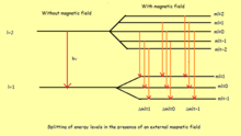
Lifting of degeneracy by an external magnetic field

In example of the strong-field Zeeman effect, when the applied field is strong enough, and then that the orbital and spin athwart momenta decouple, the skillful breakthrough numbers are at present n, fifty, m_l , and one thousand_s . Here, 50_z and South_z are conserved, so the perturbation Hamiltonian is given by-

{\hat {5}}=eB(L_{z}+2S_{z})/2m

bold the magnetic field to be forth the z-management. So,

{\hat {V}}=eB(m_{fifty}+2m_{due south})/2m

For each value of g_l , there are ii possible values of one thousand_{due south} , $\pm ane/two$ .

Stark effect [edit]

The splitting of the energy levels of an atom or molecule when subjected to an external electric field is known every bit the Stark effect.

For the hydrogen atom, the perturbation Hamiltonian is

{\lid {H}}_{south}=-|east|Ez

if the electric field is chosen along the z-management.

The energy corrections due to the applied field are given past the expectation value of ${\chapeau {H}}_{s}$ in the $|nlm\rangle$ basis. It can be shown by the selection rules that $\langle nlm_{fifty}|z|n_{1}l_{1}m_{l1}\rangle \neq 0$ when $l=l_{one}\pm 1$ and $m_{l}=m_{l1}$ .

The degeneracy is lifted only for certain states obeying the selection rules, in the first order. The first-order splitting in the energy levels for the degenerate states $|two,0,0\rangle$ and $|2,ane,0\rangle$ , both respective to n = 2, is given past $\Delta E_{2,1,m_{l}}=\pm |e|(\hbar ^{2})/(m_{east}east^{two})E$ .

References [edit]

^ ^a ^b ^c Merzbacher, Eugen (1998). Breakthrough Mechanics (3rd ed.). New York: John Wiley. ISBN0471887021. {{cite book}}: CS1 maint: uses authors parameter (link)
^ Levine, Ira Northward. (1991). Quantum Chemistry (fourth ed.). Prentice Hall. p. 52. ISBN0-205-12770-three. {{cite book}}: CS1 maint: uses authors parameter (link)
^ ^a ^b Messiah, Albert (1967). Breakthrough mechanics (tertiary ed.). Amsterdam, NLD: Northward-The netherlands. pp. 98–106. ISBN0471887021. {{cite book}}: CS1 maint: uses authors parameter (link)
^ McIntosh, Harold V. (1959). "On Accidental Degeneracy in Classical and Quantum Mechanics" (PDF). American Journal of Physics. American Association of Physics Teachers (AAPT). 27 (nine): 620–625. Bibcode:1959AmJPh..27..620M. doi:10.1119/1.1934944. ISSN 0002-9505.