How To Add Axis To Image Python

Calculation a Tertiary Y-centrality to Python Philharmonic Chart

A easily-on tutorial to create a multiple Y-axis combo chart with Matplotlib, Seaborn, and Pandas plot()

Visualizing data is vital to analyzing data. If you can't see your data — and encounter it in multiple ways you'll have a difficult time analyzing that data.

Source from Python Data [1]

At that place are many different graphs to visualize information in Python and thankfully with Matplotlib, Seaborn, Pandas, Plotly, etc., you tin can make some pretty powerful visualizations during information analysis. Amidst them, the combo chart is a combination of 2 nautical chart types (such as bar and line) on the aforementioned graph. It'due south one of Excel's most pop built-in plots and is widely used to show dissimilar types of information.

In the previous article, we take discussed how to create a dual-centrality combo chart. In some cases, information technology's very useful to add a third or more than y-centrality to visually highlight the differences between unlike sets of data. In this article, we'll explore how to add a third y-axis with Matplotlib, Seaborn, and Pandas plot(). This commodity is structured as follows:

Matplotlib
Seaborn
Pandas plot()

Please check out the Notebook for the source code. More than tutorials are bachelor from Github Repo.

For the demo, we'll utilise the London climate data from Wikipedia:

                      x            = ['Jan', 'February', 'Mar', 'Apr', 'May', 'Jun', 'Jul', 'Aug', 'Sep', 'Oct', 'Nov', 'Dec']
            average_temp            = [5.2, five.3,7.vi,9.9,13.iii,16.5,18.vii, 18.v, 15.7, 12.0, viii.0, 5.5]
            average_percipitation_mm            = [55.ii, twoscore.9, 41.six, 43.seven, 49.iv, 45.1, 44.v, 49.five, 49.1, 68.5, 59.0, 55.2]
            average_uv_index            = [i,1,2,4,5,vi,six,5,iv,2,one,0]          london_climate = pd.DataFrame(
            {
            'average_temp': average_temp,
            'average_percipitation_mm': average_percipitation_mm,
            'average_uv_index': average_uv_index
            },            
            index=x
)

It's pretty easy to plot multiple charts on the same graph. For instance, with Matplotlib, we can simply call the chart function one after another.

          plt.plot(x, average_temp, "-r", label="average temp")
plt.plot(x, average_percipitation_mm, "-b", characterization="average percipitation mm", )
plt.plot(x, average_uv_index, "-1000", label="average temp")          plt.legend(loc="upper left")
plt.show()

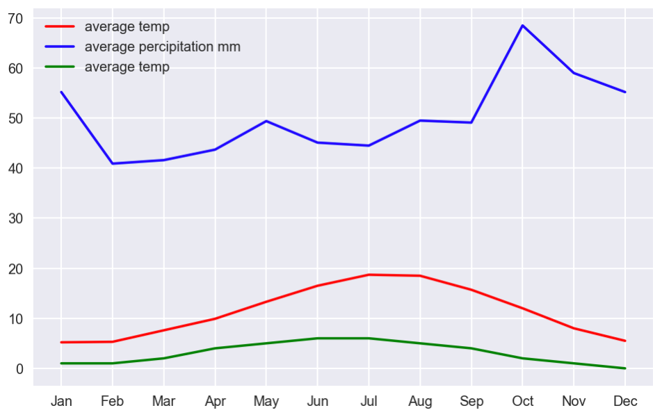
Single-centrality philharmonic chart (Image past author)

This certainly creates a combo chart, but all lines employ the same Y-centrality. It tin can exist very hard to view and interpret, especially when data are in different ranges. We tin can ameliorate it using multiple Y-axes. Just working with multiple Y-axis can be a bit disruptive at offset. Allow's go ahead and explore how to add a third Y-axis to the Python combo chart.

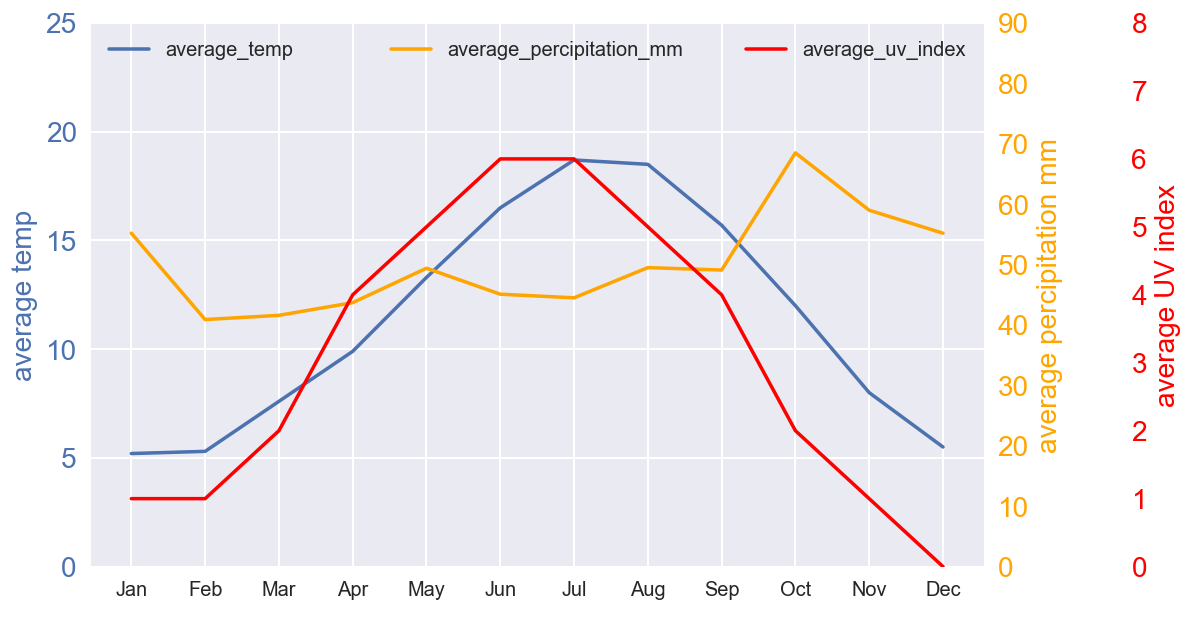
ane. Matplotlib — add the tertiary Y-axis

In the previous article, nosotros have learned the fox to make a dual-axis combo chart past calling twin() to generate ii separate Y-centrality that shares the same X-axis. Creating a third y-centrality can be done similarly by creating another twinx() axis and offsetting the 3rd centrality' correct spine position using set_postion():

          # Create effigy and axis #ane
fig, ax1 = plt.subplots()          # plot line nautical chart on centrality #ane
p1, = ax1.plot(10, average_temp)            
ax1.set_ylabel('average temp')
ax1.set_ylim(0, 25)
ax1.legend(['average_temp'], loc="upper left")
ax1.yaxis.characterization.set_color(p1.get_color())
ax1.yaxis.label.set_fontsize(14)
ax1.tick_params(axis='y', colors=p1.get_color(), labelsize=14)          # ready the 2nd axis
            ax2 = ax1.twinx()                        
# plot bar nautical chart on centrality #2
p2, = ax2.plot(x, average_percipitation_mm, color='orange')
ax2.filigree(False) # turn off grid #2
ax2.set_ylabel('average percipitation mm')
ax2.set_ylim(0, xc)
ax2.legend(['average_percipitation_mm'], loc="upper center")
ax2.yaxis.label.set_color(p2.get_color())
ax2.yaxis.label.set_fontsize(14)
ax2.tick_params(axis='y', colors=p2.get_color(), labelsize=14)          # set up the 3rd axis
            ax3 = ax1.twinx()            
# Outset the right spine of ax3.  The ticks and label have already been placed on the correct by twinx to a higher place.
            ax3.spines.right.set_position(("axes", 1.15))            
# Plot line nautical chart on axis #3
p3, = ax3.plot(ten, average_uv_index, color='ruby')
ax3.filigree(False) # plow off grid #3
ax3.set_ylabel('average UV index')
ax3.set_ylim(0, 8)
ax3.legend(['average_uv_index'], loc="upper right")
ax3.yaxis.characterization.set_color(p3.get_color())
ax3.yaxis.label.set_fontsize(14)
ax3.tick_params(centrality='y', colors=p3.get_color(), labelsize=14)          plt.bear witness()

The 1st line chart is plotted on the ax1 every bit we commonly do. We phone call ax2 = ax1.twinx() to set up the 2d axis and plot the 2d line chart. Later that, nosotros call ax3 = ax1.twinx() again to ready the tertiary centrality and plot the 3rd line chart. The play a joke on is to call ax3.spines.right.set_position(("axes", ane.15)) to first the right spine of ax3. Note that ax2.filigree(Faux) and ax3.grid(False) are chosen to avert a grid display issue. Past executing the lawmaking, yous should become the post-obit output:

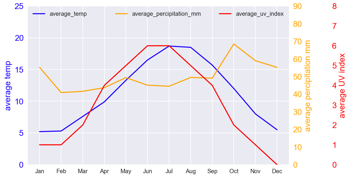
Third y-axis combo chart using Matplotlib (image by author)

3. Seaborn — add the 3rd Y-centrality

Seaborn is a high-level Data Visualization library built on meridian of Matplotlib . Backside the scenes, information technology uses Matplotlib to describe its plots. For low-level configurations and setups, nosotros can always call Matplotlib 'southward APIs, and that's the play a joke on to make a multiple Y-axis philharmonic chart in Seaborn :

          # plot line chart on axis #1
ax1 = sns.lineplot(
            10=london_climate.index,            
            y='average_temp',            
            data=london_climate,            
            sort=False,            
            color='blueish'
)
ax1.set_ylabel('boilerplate temp')
ax1.set_ylim(0, 25)
ax1.legend(['average_temp'], loc="upper left")
ax1.yaxis.characterization.set_color('blue')
ax1.yaxis.label.set_fontsize(fourteen)
ax1.tick_params(axis='y', colors='blueish', labelsize=14)          # prepare up the second centrality
            ax2 = ax1.twinx()            
# plot bar chart on axis #two
sns.lineplot(
            x=london_climate.alphabetize,            
            y='average_percipitation_mm',            
            data=london_climate,            
            sort=Simulated,            
            color='orange',            
            ax = ax2            # Pre-existing axes for the plot
)
ax2.grid(Faux) # turn off grid #2
ax2.set_ylabel('average percipitation mm')
ax2.set_ylim(0, 90)
ax2.legend(['average_percipitation_mm'], loc="upper eye")
ax2.yaxis.label.set_color('orange')
ax2.yaxis.label.set_fontsize(14)
ax2.tick_params(axis='y', colors='orange', labelsize=fourteen)          # fix the 3rd axis
            ax3 = ax1.twinx()            
# Offset the right spine of ax3. The ticks and label have already been placed on the right by twinx above.
            ax3.spines.right.set_position(("axes", ane.15))            
# Plot line chart on centrality #3
p3 = sns.lineplot(
            x=london_climate.index,            
            y='average_uv_index',            
            data=london_climate,            
            sort=Imitation,            
            color='cherry',            
            ax = ax3            # Pre-existing axes for the plot
)
ax3.grid(False) # turn off grid #3
ax3.set_ylabel('average UV index')


ax3.set_ylim(0, 8)
ax3.legend(['average_uv_index'], loc="upper right")
ax3.yaxis.characterization.set_color('red')
ax3.yaxis.characterization.set_fontsize(14)
ax3.tick_params(axis='y', colors='ruby-red', labelsize=14)          plt.prove()

sns.lineplot() returns a Matplotlib axes object ax1. Then, similar to the Matplotlib solution, we call ax2 = ax1.twinx() to set up the 2nd centrality. Afterwards that, the sns.lineplot() is called with the argument ax = ax2 to plot on the existing axes ax2. For the tertiary line, nosotros call ax3 = ax1.twinx() again to gear up the 3rd axis, and sns.lineplot() with the argument ax=ax3 to plot on the existing axes ax3. We apply the same fox ax3.spines.right.set_position(("axes", 1.15)) to offset the right spine of ax3. By executing the code, you lot should get the following output:

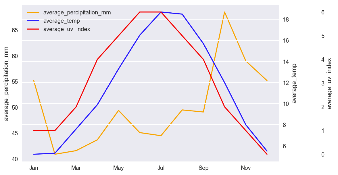
Third y-axis combo chart using Seaborn (image by writer)

iv. Pandas plot() — add the 3rd Y-axis

Pandas employ plot() method to create charts. Under the hood, it calls Matplotlib'south API by default. Nosotros tin can fix the argument secondary_y to Truthful to let the 2d chart to be plotted on the secondary Y-centrality. To add a third chart with the tertiary Y-axis, we tin apply the same trick we did earlier.

          # Create the figure and axes object
fig, ax = plt.subplots()          # Plot the beginning x and y axes:
london_climate.plot(
            use_index=True,            
            y='average_percipitation_mm',            
            ax=ax,                        
            color='orangish'
)
ax.set_ylabel('average_percipitation_mm')          # Plot the second 10 and y axes.            
# By secondary_y = True a second y-axis is requested
ax2 = london_climate.plot(
            use_index=True,            
            y='average_temp',            
            ax=ax,            
            secondary_y=Truthful,            
            color='bluish'
)
ax.legend().set_visible(Imitation)
ax2.set_ylabel('average_temp')          # Plot the third x and y axes
            ax3 = ax.twinx()
ax3.spines.right.set_position(("axes", ane.fifteen))            
london_climate.plot(
            use_index=Truthful,            
            y='average_uv_index',            
            ax=ax3,            
            color='red'
)
ax3.grid(False)
ax3.set_ylabel('average_uv_index')          # Set upward legends
ax3.fable(
            [ax.get_lines()[0], ax2.get_lines()[0], ax3.get_lines()[0]],            
            ['average_percipitation_mm','average_temp','average_uv_index'],            
            loc="upper left"
)          plt.show()

Note that nosotros set use_index=True to utilise the index as ticks for the x-centrality. By executing the code, you lot should get the post-obit output:

Third y-axis philharmonic chart using Pandas plot() (image by author)

Conclusion

In this commodity, we have learned how to create a multiple Y-axis combo chart with Matplotlib , Seaborn , and Pandas plot(). The combo chart is one of the most popular charts in Data Visualization, knowing how to create a multiple Y-axis combo chart can exist very helpful to analyzing data.

Thanks for reading. Please check out the Notebook for the source code and stay tuned if you are interested in the applied attribute of machine learning. More tutorials are bachelor from the Github Repo.

References

[1] Python Data — Visualizing information- overlaying charts in python